The point contact model and 3D friction cones

Maintaining balance is one of the crucial things for roboticists working with mobile robots, especially with humanoid robots. An example of a walking HRP-2 robot is shown in the teaser figure.

When a foot sole of HRP-2 is in contact with a surface, for example, the ground plane, the contact must remain fixed because otherwise the robot is at risk of falling. Therefore, it is of key interest to derive what we call the contact stability condition for such type of fixed contact.

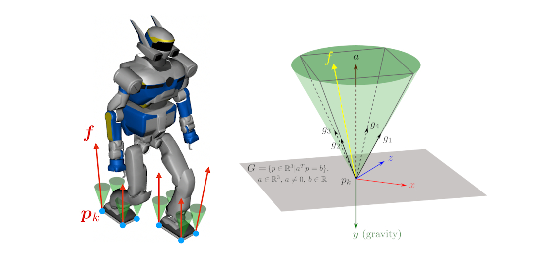
In this article, we consider the contact point $p_k$ located at the right foot sole of HRP-2 in the teaser example. We discuss the contact stability condition of this point contact model followed by its linear approximation.

Notations

The math symbols in the point contact model are illustrated in the figure below:

In particular, we define:

• Ground plane. We model the ground as a plane in Cartesian space $G = \{p\in \mathbb{R}^3|a^Tp=b\}$ with a unit normal vector $a\in \mathbb{R}^3$, $a\neq 0$, $b\in \mathbb{R}$. The coefficient of friction between the foot sole and the ground is denoted by $\mu$ ($\mu>0$).
• Contact point. Let $p_k$ be the position of a contact point $k$ located on the ground surface, i.e. $a^Tp_k=b$. We define at contact point $k$ a right-hand coordinate frame $C$ whose $xz$-plane overlaps the plane $G$ and whose $y$-axis points towards the gravity direction, i.e., the opposite direction to the ground normal $a$.
• Contact force. We use $f=(f_x, f_y, f_z)^T$ to denote the 3D contact force exerted by the ground. Let $f^n$ and $f^t$ denote respectively the normal and the tangential component of $f$:
  \begin{align} f^n &= (f\cdot a)a,\\ f^t &= f-(f\cdot a)a. \end{align}

Contact stability condition and Coulomb friction cone

To prevent the contact point from sliding, the contact force must satisfy the following conditions:

1. $f\cdot a > 0$, which means that $f$ must point from the environment (ground) to the robot.
2. $\lVert f^t\rVert \leq \mu\lVert f^n \rVert$, meaning that the magnitude of tangential force $f^t$ (which includes the friction force) can not exceed the normal force $f_n$, otherwise the contact switches to the sliding mode.

The second condition requires that the contact force $f$ lies in a second-order “ice-cream” cone, or more formally a 3D Coulomb friction cone denoted by the symbol $\mathcal{K}^3$.

In fact, the two contact-stability conditions can be unified into a single equation if we define $\theta$ as half of the apex angle of $\mathcal{K}^3$ and let $\mu=\tan\theta$. The contact-stability conditions is rewritten as
$$\lVert f^t\rVert \leq \lVert f^n\rVert\tan\theta,$$

or equivalently,
$$\lVert f-(f\cdot a)a \rVert \leq (f\cdot a)\tan\theta.$$

In the simple case illustrated in Figure 1, the ground normal $a=(0, -1, 0)^T$ and the contact-stability condition becomes:
$$\mathcal{K}^3 = \{f=(f_x,f_y,f_z)^T|\sqrt{f_x^2 + f_z^2} \leq -f_y\tan\theta\}.$$

Pyramid Approximation

For the ease of numerical optimization, it is a common practice to approximate the Coulomb friction cone $\mathcal{K}^3$ using a pyramid. For brevity, we only give the pyramid approximation for the case $a=(0, -1, 0)^T$. In this case, we define
$${\mathcal{K}^3}^\prime = \{f=\sum_{n=1}^4{\lambda_n g_n}|\lambda_n\geq 0\},$$ with

\begin{align} g_1 &= \left(\sin{\theta}, -\cos{\theta}, 0\right)^T, \\ g_2 &= \left(-\sin{\theta}, -\cos{\theta}, 0\right)^T, \\ g_3 &= \left(0, -\cos{\theta}, \sin{\theta}\right)^T, \\ g_4 &= \left(0, -\cos{\theta}, -\sin{\theta}\right)^T, \end{align}

where $g_i\ (i=1,2,3,4)$ are the 3D-generators of the pyramid.

The approximation is illustrated in Figure 2, where the friction cone $\mathcal{K}^3$ is approximated by the conic hull ${\mathcal{K}^3}^\prime$ which is spanned by 4 points on the boundary of $\mathcal{K}^3$, namely the generators $g_i$ ($i=1,2,3,4$). This approximation is a very useful linerazation technique for solving optimal control problems with point contact models.

Further discussion

Multiple point contact models can be combined to form a planar contact model, e.g. to model the contact between a foot sole of HRP-2 and the ground as shown in the teaser figure. Friction cones can be combined into wrench friction cones using polyhedral geometry.