All data points lie in a sub-manifold of the 3 dimentional space. If somehow we find this sub-manifold which can be “unfolded” to a lower dimensional space (2D space in this case), then we can reduce the dimensiontality of the data without losing much information.
Principle

Let $x$ be a $d$-dimensional random vector and $x_1$,…,$x_N$ be an i.i.d. sample of $x$. We denote by $X$ the $N\times d$ matrix (a.k.a. the \textit{design matrix} of the sample) defined by:
\begin{equation}
X = \left( \begin{array}{ccc}
\ldots & x_1^T & \ldots \\
& \vdots & \\
\ldots & x_N^T & \ldots\\
\end{array} \right).
\end{equation}
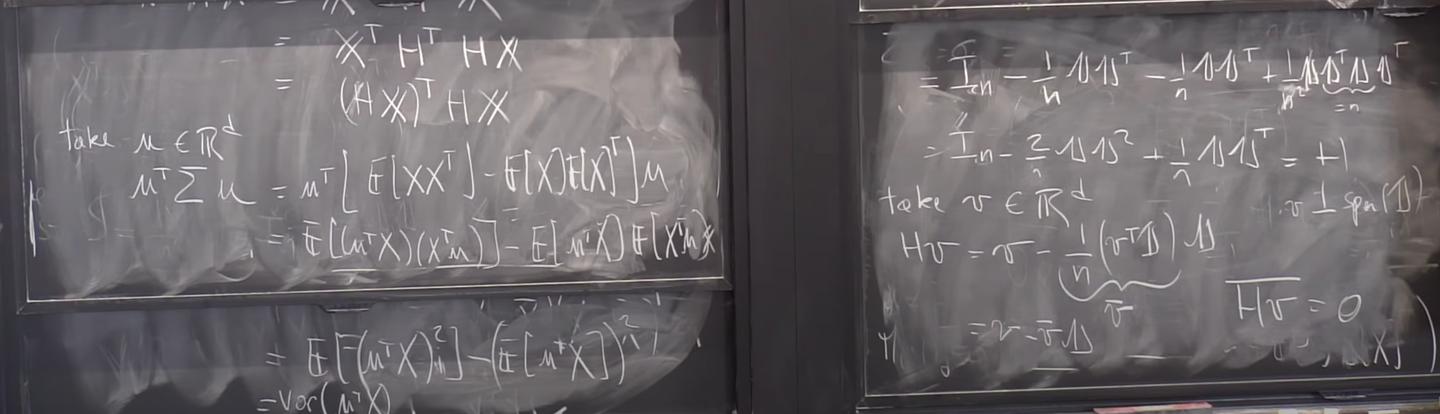
In order to perserve the information as much as possible, our idea is to find directions along which the variance of the projected data is maximal. Let $u\in R^d$, the affine transformation of the ran. vec. $x$ along $u$, i.e. $u^Tx$, is a ran. var. with variance:
\begin{align}
\text{Var}(u^Tx) =& E\left((u^Tx)^2\right) - E\left(u^Tx\right)^2 \\
=& E\left(u^Txx^Tu\right) - E\left(u^Tx\right)E\left(x^Tu\right) \\
=& u^TE\left(xx^T\right)u - u^TE\left(x\right)E\left(x\right)^Tu \\
=& u^T\Sigma u,
\end{align}
where $\Sigma=E\left(xx^T\right)-E\left(x\right)E\left(x\right)^T$ is the covariance matrix of $x$ by definition.
We would like to solve the problem
\begin{equation}
\begin{aligned}
& \underset{u\in R^d}{\text{maximize}}
& & u^T\Sigma u \\
& \text{subject to}
& & \|u\| \leq 1.
\end{aligned}
\end{equation}
Note that the constraint $|u| \leq 1$ is necessary because otherwise the problem is ill-posed: the objective function is unlimited due to unlimited scale of $u$, which is meaningless in the sense of finding the optimal direction of $u$ which optimizes $\text{Var}(u^Tx)$.
Note also that in practice, we only have an i.i.d. sample instead of the real distribution of $x$, namely, the covariance matrix $\Sigma$ in the above problem is unknown. Therefore, instead of solving the original problem, we introduce the empirical mean and the empirical covariance of the sample $x_1$,…,$x_N$:
\begin{align}
\bar{x} &= \frac{1}{N}\sum_{i=1}^Nx_i, \\
S &= \frac{1}{N}\sum_{i=1}^Nx_ix_i^T - \bar{x}\bar{x}^T,
\end{align}
and solve the new problem:
\begin{equation}
\begin{aligned}
& \underset{u\in R^d}{\text{maximize}}
& & u^TS u \\
& \text{subject to}
& & \|u\| \leq 1.
\end{aligned}
\end{equation}
Firstly, we show that objective function in the new problem is actually equal to the empirical variance of $u^Tx_i$, …, $u^Tx_N$.
\begin{align}
u^TSu =& u^T\left(\frac{1}{N}\sum_{i=1}^Nx_ix_i^T\right)u - u^T\left(\frac{1}{N}\sum_{i=1}^Nx_i\frac{1}{N}\sum_{i=j}^Nx_j^T\right)u \\
=& \frac{1}{N}\sum_{i=1}^Nu^Tx_ix_i^Tu - \frac{1}{N}\sum_{i=1}^Nu^Tx_i\frac{1}{N}\sum_{i=j}^Nx_j^Tu \\
=& \frac{1}{N}\sum_{i=1}^N(u^Tx_i)^2 - \left(\frac{1}{N}\sum_{i=1}^Nu^Tx_i\right)^2
\end{align}
which is by definition the empirical variance of $u^Tx_i$, ..., $u^Tx_N$.
See [2] for more information about the empirical covariance matrix $S$.
Then we show how to solve the new problem. The Lagrangian of the problem is
\begin{align}
L(u,\lambda) = u^TSu - \lambda(u^Tu-1).
\end{align}
The partial derivitavie w.r.t. $u$ is
\begin{align}
\frac{\partial L}{\partial u} = 2(Su-\lambda u)
\end{align}
From $\frac{\partial L}{\partial u}=0$ we obtain
\begin{align}
Su=\lambda u
\end{align}
which means the optimal $\lambda$ and $u$ must be an eigenvalue and the corresponding eigenvector of $S$. Since $u^TSu$ is equal to empirical variance, it means that $u^TSu\geq0$ for any $u\in R^d$. Therefore, the symmetric matrix $S$ is positive semi-definite, and hence is diagonalizable. Therefore, the new problem is a convex optimization problem (with concave objective function). The optimal solution $u^*$ is the eigenvector of the first (i.e. largest) eigenvalue of $S$.
PCA algorithm

References
- Ali Ghodsi. Lec 3: QDA, Principal Component Analysis (PCA). 2015.
- Philippe Rigollet. Lecture 19: Principal Component Analysis. https://youtu.be/WW3ZJHPwvyg, 2017.